How to turn an LLM into a low-latency classifier on the fly

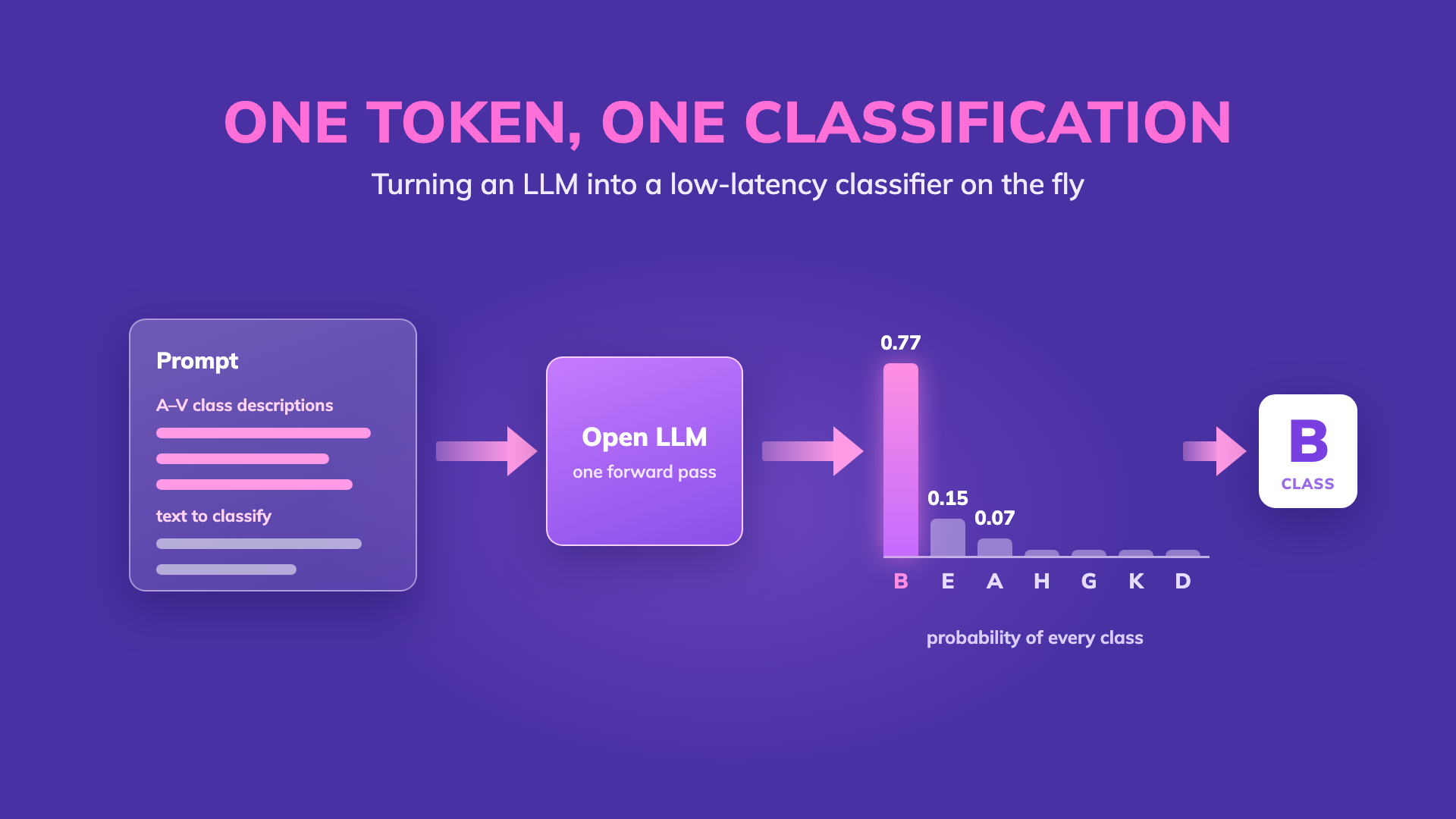
Many applications rely on multi-class text classification, which assigns each input to exactly one class from a fixed set. Dedicated services such as Jev, a closed-source API built specifically for classification, are fast because they return a class and a confidence score rather than generated text. It is well known that a general-purpose language model can do the same. What is used less outside machine learning is two by-products of the same forward pass: the probability of every class, and a confidence score read from those probabilities.

The technique requires no fine-tuning, no classification head and no output parser: the prompt describes the classes and asks for a one-letter answer, and a single forward pass returns the probability of every class. Below we walk through the recipe in two steps and measure it on one task, routing cybersecurity prompts. On that task, two Gemma models match Jev's accuracy and answer with lower latency at light load. Their confidence score is 1 − p₂, one minus the runner-up class's probability. Escalate the least confident classifications by this score and the Gemma models' error rate on the rest keeps falling, past the point where Jev's own confidence score stops lowering Jev's.

The recipe

Step 1: Describe the classes and read their probabilities from one token

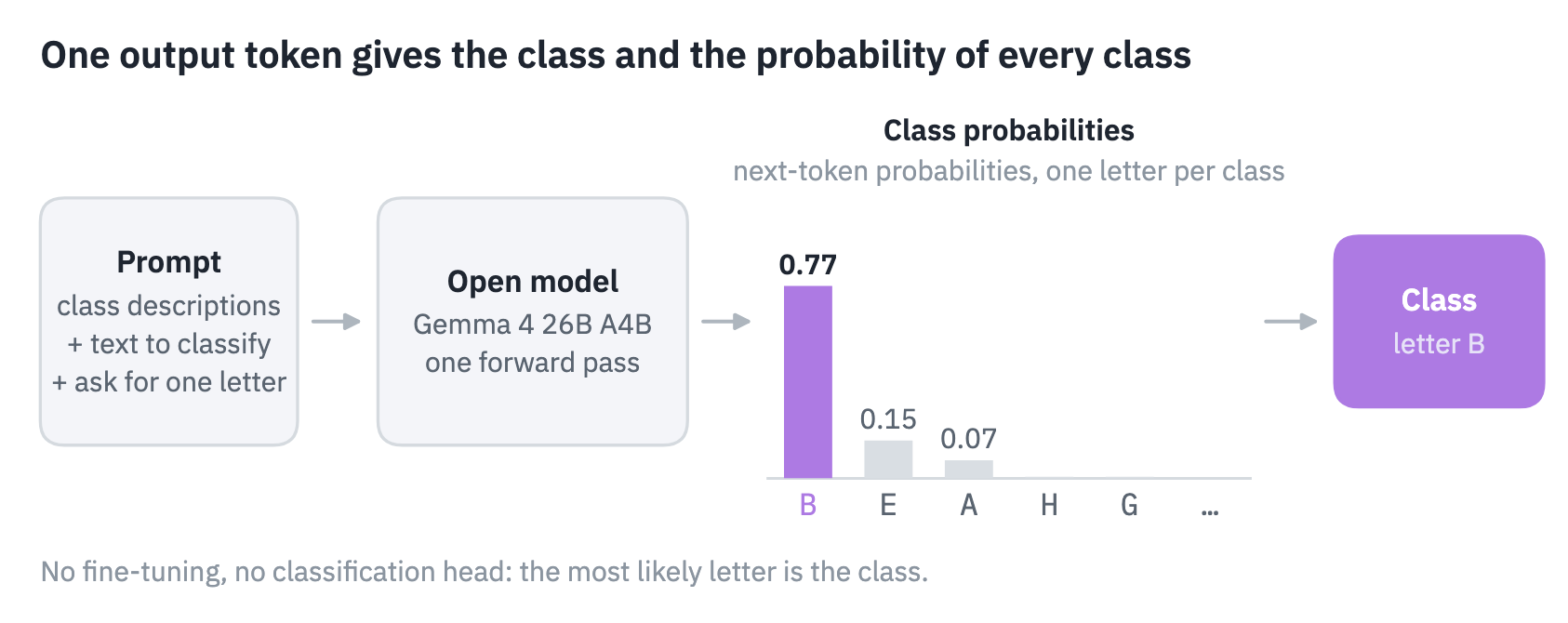
Give each class a single capital letter, A to V for our 22 classes, and describe each class in the prompt, including what does not belong in it and how to tell it apart from classes it is easily confused with.¹ The text to classify follows, with an instruction to answer with one letter. Then have the model generate exactly one token and read the probability it assigns to each letter.² In the figure, B has the highest probability, 0.77, and is the predicted class. Each classification costs one forward pass, as with a dedicated classifier.

Step 2: Read a confidence score and set an escalation threshold

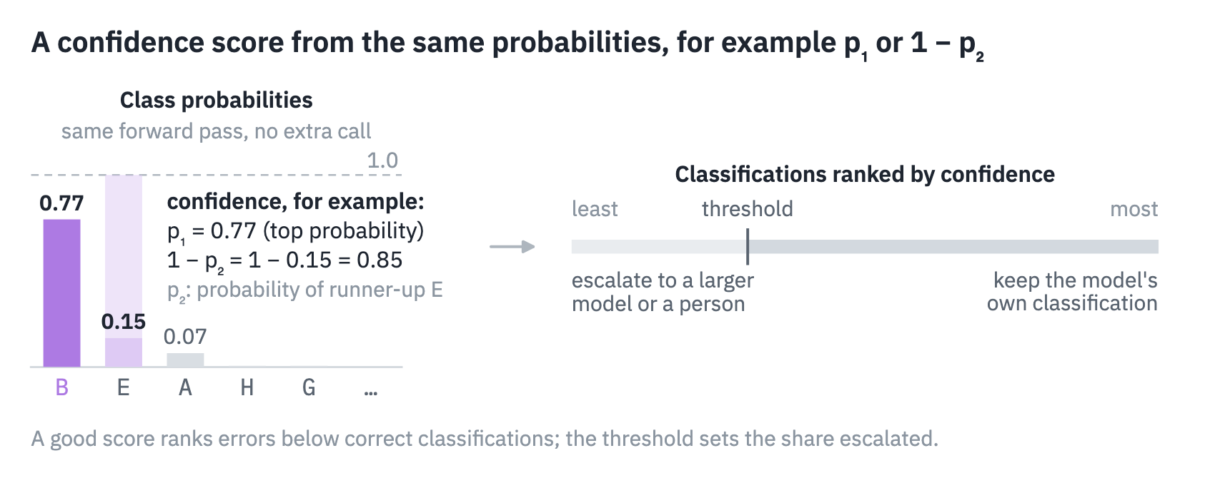
The same probabilities also measure how decisive the model was. Several confidence scores can be read from them, for example the top probability p₁ or one minus the probability of the runner-up class, 1 − p₂; the results section compares the two. To decide what to escalate, rank the classifications by the chosen score and send those below an escalation threshold to a larger model or a human reviewer, as the right half of the figure shows.³ The error rates we report under escalation in the results cover only the model's own answers on the classifications it keeps: escalated classifications are left out of the count, and no answer from a larger model or a reviewer is included.

Results: routing cybersecurity prompts

Our router assigns each incoming cybersecurity prompt to one of 22 task groups and dispatches it to the model best suited to that group. We compared three classifiers on the same labeled held-out set, each receiving identical input text:

• Gemma 4 26B A4B, Google's open mixture-of-experts model, used as released.⁴
• Gemma 4 E2B, a small language model (SLM) we had already trained with reinforcement learning as a language model that writes out its reasoning, not as a classifier; here it is read exactly like the 26B: one output token, no generated reasoning.⁵
• Jev, called through its API.

In deployment we read the E2B the same way and use it as a fast task-drift check within agentic sessions, while the primary router can be a different model. Each Gemma model was served on a single NVIDIA GH200 GPU.⁶

Accuracy and latency

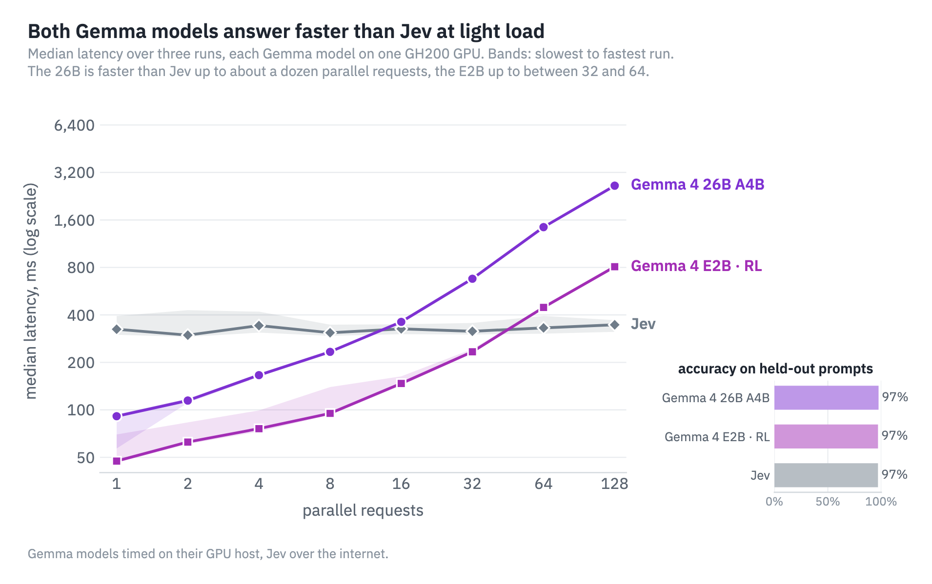
The three classifiers are on par in accuracy, measured on every held-out prompt with nothing escalated: 97% for Gemma 4 26B A4B, for Jev and for Gemma 4 E2B. With one request in flight, the median latency is 91 ms for the 26B and 47 ms for the E2B, against 325 ms for Jev. As parallel requests grow, each model's GPU saturates and requests queue; even so, the 26B's median latency stays below Jev's up to about a dozen parallel requests, and the E2B's up to a point between 32 and 64.

Throughput

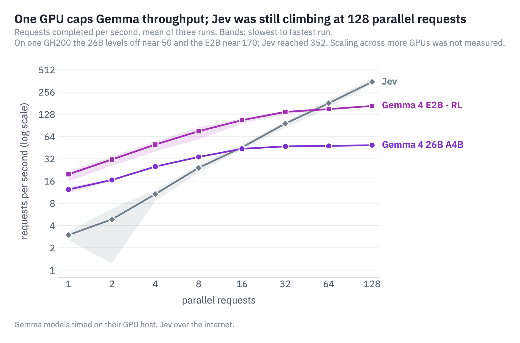
On one GH200, throughput levels off at about 50 requests per second for the 26B and about 170 for the E2B; Jev's was still rising, at 352 requests per second at 128 parallel requests, the highest load shown. The Gemma ceiling is the hardware we allocated, not the method. More GPUs or replicas would raise it; we did not measure that.

Probability on the letters

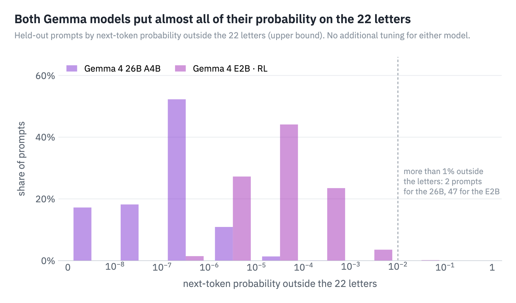
A confidence score read from the letters is meaningful only if the next-token distribution puts nearly all of its probability mass on them, and the figure shows that both Gemma models do. For the median held-out prompt, about 2 in 10 million of the 26B's probability mass falls outside the letters, and about 3 in 100,000 of the E2B's. Fewer than 0.2% of prompts put more than 1% outside the letters for either model, with no additional tuning. Thus, the letter probabilities can be read as returned.⁷

Confidence and escalation

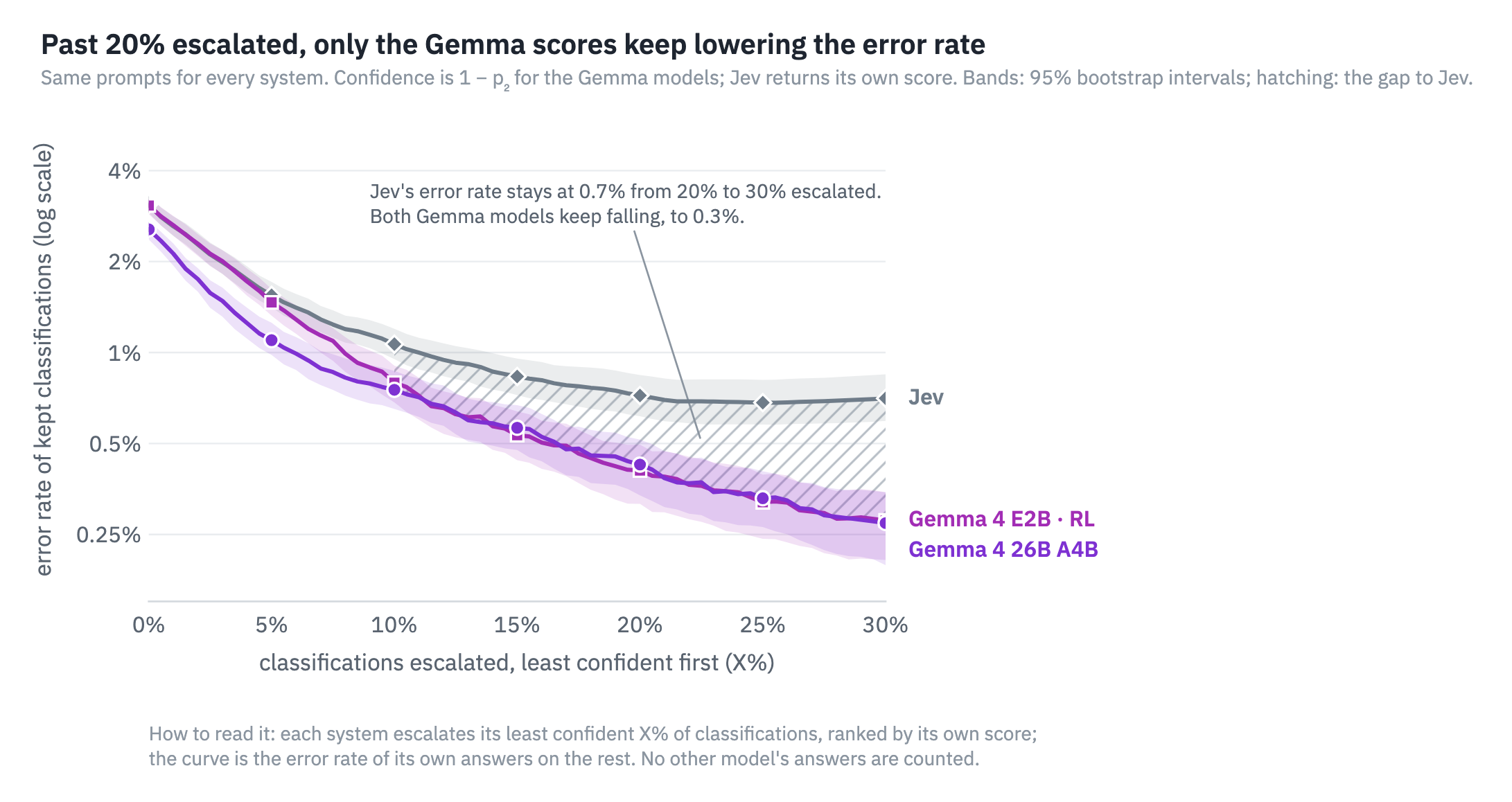
Jev returns its own confidence score, so for each system we escalate its least confident X% of classifications by its own score (the figure's x axis) and measure the error rate of its own classifications on the prompts it keeps. The escalated prompts are removed from the measurement rather than passed to a larger model, so the curves show how well each score separates a model's errors from its correct answers, not the accuracy of a system that includes a larger model.⁸ With nothing escalated, that error rate is 2.6% for the 26B and 3.1% for both Jev and the E2B; escalating the least confident 10% lowers it to 0.8%, 1.1% and 0.8%. Jev's error rate stays at 0.7% from 20% to 30% escalated: in that range its score is escalating classifications that are no more likely to be wrong than the ones it keeps. Under 1 − p₂, the error rate of the classifications the 26B and the E2B keep continues to fall, to 0.3% at 30% escalated.

We rank the Gemma models' classifications by 1 − p₂ rather than p₁ mainly because most errors are confusions between two classes: when the 26B was wrong, the correct class was ranked second 93% of the time, so the runner-up's probability carries the signal. On this task, however, the two scores rank classifications almost identically.⁹

Choosing a model

Smaller off-the-shelf models were clearly less accurate with our class descriptions, which we wrote while working with the 26B. A small model already trained for the domain, such as our E2B, closes that accuracy gap and serves more than three times the 26B's requests per second on one GPU; without one, a mid-size open model such as the 26B matches Jev's accuracy with no training at all.

Takeaways

• Any open LLM or SLM can act as a classifier on the fly: describe the classes, have the model generate one token and read the class probabilities, with no fine-tuning and no output parsing. Serving the model still needs a GPU or an API.
• An off-the-shelf open model can match a purpose-built classification API on accuracy and, at light load, answer with lower latency.
• The same forward pass also yields a confidence score. On our task, escalating by 1 − p₂ kept lowering the Gemma models' error rate on the classifications they keep, past the point where the closed API's own score stopped lowering Jev's.
• Throughput under heavy load is determined by the hardware allocated, not by the method.
• The choice of model matters more than the recipe, so measure candidate models on your own classes before relying on one.